R Regression Diagnostics Part 1
Linear regression can be a fast and powerful tool to model complex phenomena. However, it makes several assumptions about your data, and quickly breaks down when these assumptions, such as the assumption that a linear relationship exists between the predictors and the dependent variable, break down. In this post, I will introduce some diagnostics that you can perform to ensure that your regression does not violate these basic assumptions. To begin with, I highly suggest reading this articleon the major assumptions that linear regression is predicated on.
We will make use of the same variables as we did in the [intro to ensemble learning](http://viksalgorithms.blogspot.com/2012/01/intro-to-ensemble- learning-in-r.html) post:
set.seed(10)
y<-c(1:1000)
x1<-c(1:1000)*runif(1000,min=0,max=2)
x2<-(c(1:1000)*runif(1000,min=0,max=2))^2
x3<-log(c(1:1000)*runif(1000,min=0,max=2))
Note that x2 and x3 are significantly nonlinear by design(due to the squared and log modifications), and will cause linear regression to make spurious estimates.
Component residual plots, an extension of partial residual plots, are a good way to see if the predictors have a linear relationship to the dependent variable. A partial residual plot essentially attempts to model the residuals of one predictor against the dependent variable. A component residual plot adds a line indicating where the line of best fit lies. A significant difference between the residual line and the component line indicates that the predictor does not have a linear relationship with the dependent variable. A good way to generate these plots in R is the car package.
library(car)
lm_fit<-lm(y~x1+x2+x3)
crPlots(lm_fit)
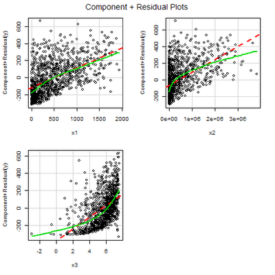
Your plot should look like this:
 Looking at the plot, we see that 2 of the predictors(x2 and x3) are significantly non-normal, based on the differences between the component and the residual lines. In order to “correct” these differences, we can attempt to alter the predictors. Typical alterations are sqrt(x), 1/x, log(x), and n^x. In this situation, we already know how the data are nonlinear, so we will be able to easily apply the appropriate transformation. In a “real-world” situation, it may take trial and error to come up with an appropriate transformation to make the predictor appear more linear. If none of the transformations work, you may have to consider not using the predictor, or switching to a nonlinear model.
library(car)
lm_fit<-lm(y~x1+sqrt(x2)+exp(x3))
crPlots(lm_fit)
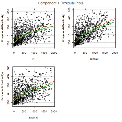
The above code modifies the linear model by using the square root of x2 as a predictor, and e^x3 as a predictor, which cancel out the squared transformation on x2 and the natural log transformation on x3, respectively. Your plot should look like this:
 As you can see, this plot shows a much more linear relationship between x2 and y and x3 and y. However, the component and residual lines for the predictors x1, x2, and x3 do not show a perfect overlap. We will look more into this in a later post.
