Mapping US Radiation Levels in R
I have posted previously about the open data available on Socrata (https://opendata.socrata.com/), and I was looking at the site again today when I stumbled upon a listing of levels of various radioactive isotopes by US city and state. The data is available at https://opendata.socrata.com/Government/Sorted-RadNet-Laboratory-Analysis /w9fb-tgv6 . You will need to click export, and then download it as a csv.
I was struck by how the data was in a very nice format for analysis. I initially wanted to look at summary statistics, but I have wanted to try some mapping for a while now, and this seemed like the right time.
Reading in the Data
To begin exploring and mapping the data, we first need to download it. After downloading, it can be read in using the read.csv command:
rad_levels<-read.csv("Sorted_RadNet_Laboratory_Analysis.csv",
stringsAsFactors=FALSE,strip.white=TRUE,header=TRUE,quote="")
This gives us a nice data frame where each row is an observation of a different type (Drinking Water, Precipitation, etc), and the columns contain location data and data on levels of various isotopes.
Associating Coordinates with the Data
Unfortunately, we are not provided with any coordinates, and in order to map this data, we will need to figure out the coordinates associated with each observation. Thankfully, I recently wrote a quick function to map place names to coordinates.
does_zip_exist<-function()
{
zip_exists<-FALSE
if(exists("zips"))
{
 zip_exists<-TRUE
 if(!nrow(zips)==43623)
 zip_exists<-FALSE
}
zip_exists
}

get.coordinates.name<-function(city,state)
{
city<-tolower(city)
state<-tolower(state)
if(!does_zip_exist())
 load("zips.RData",.GlobalEnv)
if(nchar(state)==2)
{
zip_row<-head(zips[zips$state_abbr==state & zips$city %in% city,],1)
}else
{
zip_row<-head(zips[zips$state %in% state & zips$city %in% city,],1)
}
if(nrow(zip_row)==0)
 zip_row<-c("NA",00000,rep("NA",4),rep(0,3))
zip_row
}
These two functions together will enable you to get the coordinates of a given US city and state. They both depend on a file called zips.RData, which can be downloaded at http://dl.dropbox.com/u/20597506/zips.RData . The file must be present in your R working directory for the functions to work. I wrote these functions really quickly, and don’t feel like rewriting them now, so please feel free to improve their performance if you want. I will make a longer post about them later if needed.
Now, we have our radiation data, and the ability to associate the place names in the data to coordinates. What we need to do now is to perform that association.
rad_level_coords<-apply(rad_levels,1,function(x) get.coordinates.name(x[2],x[1]))
rad_level_coords<-do.call(rbind,rad_level_coords)
rad_level_frame<-cbind(rad_levels,rad_level_coords)
This code will take each row of the radiation levels data and find the coordinates associated with the place name. It will then combine the coordinate data into a data frame, and merge it with the radiation data.
Cleaning up the Data
One problem at this stage is that some of the place names in the radiation data will not properly map to coordinates. The get.coordinates.name function outputs a zip code of 00000 in this case. Thus, we can remove rows that do not have proper coordinates by filtering out the rows with a zip code of 00000.
rad_level_frame<-rad_level_frame[rad_level_frame$zip!=00000,]
We can also check the classes of the columns in rad_level_frame to ensure that the coordinates are numeric.
sapply(rad_level_frame,class)
Unfortunately, they are not numeric columns, and they will need to be in order to use them to generate a map, so we will need to convert them:
rad_level_frame$lat<-as.numeric(rad_level_frame$lat)
rad_level_frame$long<-as.numeric(rad_level_frame$long)
Setting up the Map
We now need to do some preliminary setup before we get started on making the map. We need to define which type(s) of measurements that we want to plot, and what isotope levels that we want to plot. For this first plot, we will look at I-131 in drinking water.
types<-c("Air Cartridge","Air Filter","Drinking Water","Precipitation","Milk")
current_type<-types[3]
target<-rad_level_frame$I.131
The types variable simply lists the types of measurements that are in the radiation data for convenience, and the current_type and target variables will allow us to simplify the code a bit.
Since we want to plot the different levels of radiation in Drinking Water, it will help if we can bin the variable. Binning allows us to split up an interval into discrete units. In this case, binning will help us by changing the target variable into a set of colors. These colors will range from “green” (least radioactive) to red (most radioactive), and will allow us to plot the data.
binned_target<-cut(as.numeric(target[target!="Non-detect" &
rad_level_frame$Sample.Type %in% current_type]),
breaks=5, labels=c("green","blue","yellow","orange","red"))
Cut is a function that will create a factor from a continuous numeric variable. Note that we have filtered out the instances of the target where nothing could be detected by removing the target variable when its value is “Non-detect”. This could also be handled by changing the “Non-detect” to a zero, but as it is unclear whether “Non-detect” means a zero value, or whether it indicates equipment failure or something else, it is best to remove it entirely. We have also removed observations where the measurement type is not “Drinking Water”. This will ensure that we only plot observations of drinking water radiation levels. Breaks specifies that we want to separate the data into 5 categories, which have been assigned labels according to the color that they will be plotted in.
Mapping the Data
Now, we are ready to create our base plot of the United States:
plot(as.numeric(zips$long[zips$long< -60]),
as.numeric(zips$lat[zips$long< -60]),
type="p",col="gray40",pch=20,cex=0.2,xlab="",ylab="")
This will plot all the longitudes and latitudes from the zips.RData file in a gray color, which gives us a good US map. Specifying that the longitude be under -60 removes some of the island possessions of the US, which unnecessarily stretch out the map. The gray provides a good neutral color over which to plot our radiation levels. The pch option gives us a closed circle plotting symbol, and the cex option makes the individual points fairly small.
Now, we are ready to plot our radiation levels over the base map:
points(as.numeric(rad_level_frame$long[target!="Non-detect"&
 rad_level_frame$Sample.Type %in% current_type]),
as.numeric(rad_level_frame$lat[target!="Non-detect"&
rad_level_frame$Sample.Type %in% current_type]),
type="p",col=as.character(binned_target),pch=20,cex=1)
The points function adds points to a plot generated by the plot function. We have only plotted the latitudes and longitudes for the radiation level observations which are not “Non-detect”, and which match our type, which is “Drinking Water”. We also set the color (col) using the binned_target variable that we created earlier. The cex value is set higher so that the points appear large relative to the map.
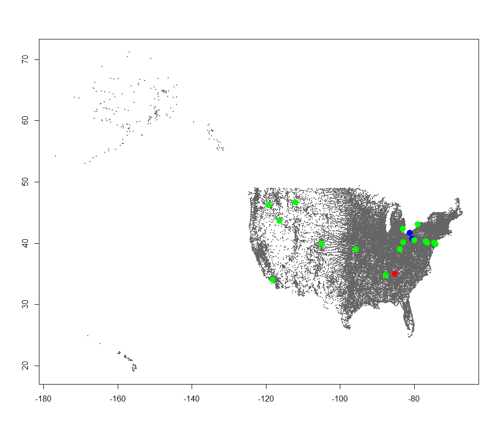
We should end up with this:
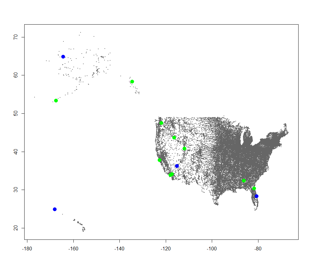
Drinking Water Radiation Map  We can change our current_type variable and run the plotting again to generate the rest of the plots: Air Filter Radiation Map
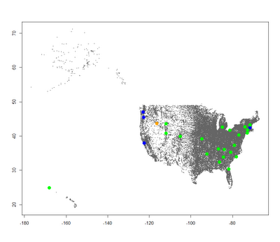
  Precipitation Radiation Map
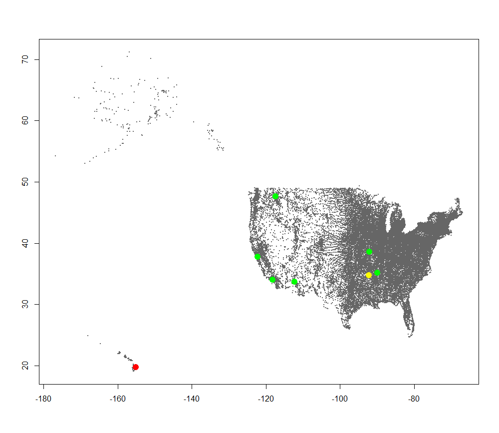
  Milk Radiation Map
  You can do more mapping with the other targets if you wish at this point. Here is the full code:
setwd("~")
rad_levels<-read.csv("Sorted_RadNet_Laboratory_Analysis.csv",
stringsAsFactors=FALSE,strip.white=TRUE,header=TRUE,quote="")
rad_level_coords<-apply(rad_levels,1,function(x) get.coordinates.name(x[2],x[1]))
rad_level_coords<-do.call(rbind,rad_level_coords)
rad_level_frame<-cbind(rad_levels,rad_level_coords)

rad_level_frame<-rad_level_frame[rad_level_frame$zip!=00000,]
rad_level_frame$lat<-as.numeric(rad_level_frame$lat)
rad_level_frame$long<-as.numeric(rad_level_frame$long)
types<-c("Air Cartridge","Air Filter","Drinking Water","Precipitation","Milk")
current_type<-c(types[5])
target<-rad_level_frame$I.131

binned_target<-cut(as.numeric(target[target!="Non-detect" &
rad_level_frame$Sample.Type %in% current_type]), breaks=5,
 labels=c("green","blue","yellow","orange","red"))

plot(as.numeric(zips$long[zips$long< -60]),
as.numeric(zips$lat[zips$long< -60]),type="p",col="gray40",
pch=20,cex=0.2,xlab="",ylab="")

points(as.numeric(rad_level_frame$long[target!="Non-detect"&
rad_level_frame$Sample.Type %in% current_type]),
as.numeric(rad_level_frame$lat[target!="Non-detect"&
rad_level_frame$Sample.Type %in% current_type]),type="p",
col=as.character(binned_target),pch=20,cex=2.5)
