Analyzing Federal Bailout Recipients in R
I was searching for open data recently, and stumbled on Socrata. Socrata has a lot of interesting data sets, and while I was browsing around, I found a data set on federal bailout recipients. Here is the data set. However, data sets on Socrata are not always the most recent versions, so I followed a link to the data source at Propublica, where I was able to find a data set that was last updated on January 17, 2012. I downloaded the data in csv format. In the rest of this post, I will perform basic analysis on this data, and show that R can be used to do the same analysis as Excel in a much simpler and more powerful way.
The data contains several columns, the most salient of which are the name of the company, its location, its industry, the amount of bailout funds received, and the amount repaid.
First, we read in the data:
bailout<-read.csv(file="bailout.csv",head=TRUE,sep=",", stringsAsFactors=FALSE,strip.white=TRUE)Next, we generate a variable called owed that calculates how much the company owes the government, or how much the government has made in profit from the company, and create a new data frame that is sorted based on how much is owed the government:
bailout<-transform(bailout,owed=bailout$total_disbursed -bailout$total_revenue-bailout$total_payback) ordered_bailout<-bailout[with(bailout,order(-owed)),]Now, we can use ggplot2 to create a nice looking bar chart, and use dev.copy() to export it(you do not need to run the last two lines, as they are solely for exporting the chart):
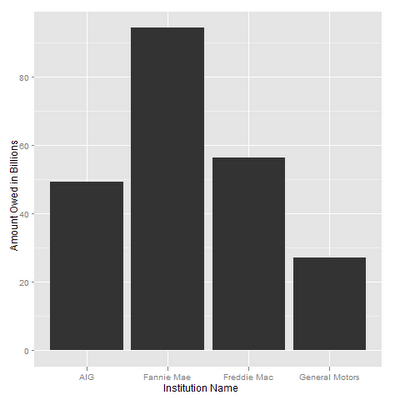
library(ggplot2) qplot(name,weight=owed/1e9, data = ordered_bailout[1:4,], geom = "bar", xlab = "Institution Name",ylab="Amount Owed in Billions") dev.copy(png,"most_owed.png") dev.off()This results in this chart:
As you can see, Fannie Mae, Freddie Mac, GM, and AIG all still owe huge amounts of money to the government. Now, we look at the top companies that the government made a profit from:
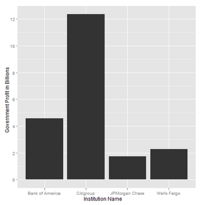
qplot(name,weight=abs(owed/1e9), data = tail(ordered_bailout,4), geom = "bar", xlab = "Institution Name", ylab="Government Profit in Billions") [](https://vik-affirm-assets.s3-us-west-1.amazonaws.com/most_repaid.png)As we can see, banks have given the government a significant profit. When we look at the sum of the money owed to the government, we see that 242.81 billion dollars have yet to be repaid:
sum(ordered_bailout$owed)/1e9Using the tapply function reveals the following(each heading is a sector name, and the number below is how much they owe the government in billions):
tapply(bailout$owed/1e9,bailout$category,sum) Bank FHA Refinance Fund -11.36362217 0.05000000 SBA Security Purchases State Housing Orgs 0.06002858 0.65537461 Mortgage Servicer Financial Services Company 1.93507502 10.47640782 Investment Fund Auto Company 13.32980009 28.53374026 Insurance Company Government-Sponsored Enterprise 48.36100458 150.77000000As you can see, the government sponsored enterprises(Fannie Mae and Freddie Mac), and the insurance companies(primarily AIG), owe the most while the banks have made a profit for the government. I will not inject any analysis into this, as we are only looking at the numbers here.
Now, we will look at how much is owed by the top 10 states:
states<-sort(tapply(bailout$owed/1e9,bailout$state,sum)) qplot(tail(names(states),10),weight=tail(states,10)) bailout[bailout$state=="PR",]$name [1] "Popular, Inc." "First BanCorp" [3] "RG Mortgage Corporation" "Scotiabank de Puerto Rico" [5] "Banco Popular de Puerto Rico"Apparently the banking sector in Puerto Rico did not do well in the financial crisis!
I noticed an interesting column in the data called “is_stress_tested”, which took on a false value, a true value, or a NULL value. I am not an expert on banking, and if someone can please shed more light on the stress test, I would appreciate it, but I believe that stress testing is a method that discovers how prone to failure the institution is.
Now, when we see how much money the institutions that have had stress testing performed versus those that have not owe, we get the following:
tapply(bailout$owed/1e9,bailout$is_stress_tested,sum) false true 13.31646 242.71883 -13.22748 This tells us that institutions that have not been stress tested owe 242 billion to the government, whereas those that have been stress tested have made a profit of 13.2 billion for the government. I am not sure if stress testing can be performed on an institution like Fannie Mae, but it seems odd that the testing has not been done on those institutions that collectively owe 242 billion dollars.
Finally, looking at the percentage of disbursed funds that are still outstanding by sector reveals the following(each heading is a sector name, and the number below is the percentage of the bailout funds that they still owe):
sort(tapply(bailout$owed,bailout$category,sum)/ tapply(bailout$total_disbursed,bailout$category,sum)) Bank SBA Security Purchases -0.04811175 0.16305670 Auto Company Financial Services Company 0.46090662 0.46762480 Insurance Company Government-Sponsored Enterprise 0.66995920 0.82478118 Investment Fund FHA Refinance Fund 0.84152859 1.00000000 Mortgage Servicer State Housing Orgs 1.00000000 1.00000000In general, it appears that Investment Funds, Government-Sponsored Enterprises, and Insurance Companies have been poor at repaying the money they were lent. The high values for Government Sponsored Enterprises and Insurance Companies are explained by the high outstanding amounts from Fannie Mae, Freddie Mac, and AIG, but the trend in Investment Funds in more interesting. Despite relatively small bailouts(and I emphasize the relatively, because 15.8 billion dollars were disbursed to Investment Funds), it appears that money has been extremely slow to come back to the Government, with 84% of the funds still outstanding.
With that, I conclude this post. I hope that this has shown you how simple data analysis can be done in R in an quick and efficient manner, and I hope that I have also been able to do interesting analyses and draw interesting facts from this data.

